Working with Data
TODO Figure out primitive list structure of
- numpy array
- pandas DataFrame
Data Science
Tools
- Python
- Pandas - working with table data
- Numpy - working with matrix structures
- Plotly
pip install plotlyconda install -c plotly plotly
- RFPImp
pip install rfpimpconda install -c conda-forge rfpimp
- Tensorflow
pip install tensorflowconda install -c conda-forge tensorflow
Info:
For zsh, one needs to include this in .zshrc
source /.bash_profile
Pandas
import pandas as pd
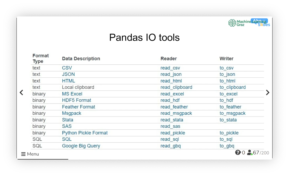
Reading and writing
Data Formats
- CSV - comma-separated values
- XLSX - Excel (based on XML)
- JSON - JavaScript Object Notation
- HTML
CSV Structure
ID, Name, Age, City
0, Tim, 25, Vienna
1, Angelica, 29, Bern
2, Alex, 31, Milano
Separators
,– typically comma-separated values;– Excel output\t#
Read a CSV file (into a pd.DataFrame)
import pandas as pd
df = pd.read_csv('example.csv', sep=';')
df
Read a XLSX file (into a pd.DataFrame)
import pandas as pd
df = pd.read_excel('example.xlsx', sheet_name='Sheet1')
df
Read a JSON file (into a pd.DataFrame)
import pandas as pd
df = pd.read_json('example.json')
df
DataFrame
Obtain (rows, columns)
df.shape
Show first 5 rows of data
df.head()
Get column names
df.columns
Drop any duplicates (overwrite df)
df = df.drop_duplicates()
Drop NaN values
df = df.dropna()
Sum not-a-number values
df.Price.isna().sum()
Sum "null" (no-value) values
df.isnull().sum()
Check sum (to check whether data was transferred completly, without corruption)
df.numberDataColumn.sum()
Check occurrences of values
df.jobs.unique()        # list of unique values
df.jobs.nunique()       # number of unique values
df.jobs.count()         # count values
df.jobs.value_counts()  # list & number of values
df.income.value_counts()/df.income.shape[0] # relative number of values
Univariate analysis of data in column
df.age.describe()  # statistics like mean, min/max etc.
df.age.median()    # median
df.age.mean()      # mean
df.age.min()       # min
df.age.max()       # max
Impute missing values with most frequent value
categorical_columns_missing = ["Gender", "Married"]

impute_missing = SimpleImputer(missing_values=np.NaN, strategy='most_frequent')

df[categorical_columns_missing] = impute_missing.fit_transform(df[categorical_columns_missing])
with mean value
impute_missing = SimpleImputer(missing_values=np.NaN, strategy='mean')

df["Amount"] = impute_missing.fit_transform(df[["Amount"]])
Queries in Pandas
df[df.job == "engineer"]
Query for data in a column
developers = df[df.job.isin(["developer", "programmer"])].index
wealthy    = df[df.income > 50000].occupation
wealthySalesperson = df[(df.occupation == "Salesperson") & (df.income > 50000)].shape[0]
Delete column(s)
df = df.drop(labels='Jobs', axis=0)     # axis=0 deletes row
df = df.drop(['Col1', 'Col2'], axis=1)  # axis=1 deletes column
Create new column
df["capital"] = df.capital_gain - df.capital_loss
Multiply the whole DataFrame by factor and round (e.g. fraction to percent)
df *= 100
df = df.astype(float).round(1)
Rename last column
df.columns = list(df.columns.values[:-1]) + ["newName"]
Replace entries
Example: Save lines to variable; Use lines to rewrite the values in the "job" column
engineers = df[df.job == "engineer"].index
engineers = df.loc[engineers, "job"] = "Engineer"
Replace
df.replace(to_replace = ["A", "B"], value ="AB")
df.replace(to_replace = np.nan, value = -1)
Replacing commas
df.apply(lambda x: x.str.replace(',','.'))
Sort
df.sort_values(by="price")
df.sort_values(by=["AveragePrice"])
Group by
Group by values in column
df.groupby("name")
df.groupby(["name", "age"])
returns groupby object (not a DataFrame!) that accepts manipulations such as mean() etc.
df.groupby(["occupation"]).salary.mean()
df.groupby(["occupation"]).salary.min()
df.groupby(["firstCategory", "secondCategory"]).count()["id"]
Reset index (to get back a DataFrame)
df.groupby(["occupation"]).salary.mean().reset_index()
Get one of the groups
df_group = df.get_group("GroupA")
Creating a DataFrame
Create DataFrame
df = pd.DataFrame({
                    'Year'  : year_list,
                    'Month' : month_list,
                    'Day'   : day_list
                  })
Create DataFrame with specified rows and columns
df = pd.DataFrame(index=['row1', 'row2', ...], columns=['column 1', 'column 2'])

for row_key in df.index:
  df[row_key] = [column_1[row_key], column_2[row_key]]
Loop through rows in DataFrame
for i, row in df.iterrows():
    print(df['Column1'][i])
    print(row['Column1'])
DataFrame from dictionary
data = {'name': [name], 'money': [money]}
df = pd.DataFrame(data, columns=["name", "money"])
Split a DataFrame
df_first500 = df.iloc[:500, :,]
df_501up    = df.iloc[500:, :,]
Pandas and NumPy
import pandas as pd
import numpy as np
create data frame
data = {
    'name': ['Eric', 'Lisa', 'John'],
    'age': [38,25,44],
    'salary': [13000, 2000, 8000]
}
df = pd.DataFrame(data)
data frame --> numpy array
np_array = df.to_numpy()
single column --> numpy array
np_array = df['age'].to_numpy()
multiple columns --> numpy array
np_array = df[['age', 'salary']].to_numpy()
integer valued columns --> numpy array
df.select_dtypes(include=int64).to_numpy()
Numpy
import numpy as np
Mean
np.mean(list_of_numbers)
Matplotlib
import matplotlib.pyplot as plt
Simple Pandas Visualisation
Histograms (1D, univariate)
df.age.hist()
Count Plot (1D, univariate)
df.workclass.value_counts().plot(kind="bar")
Scatter Plot (2D, bivariate)
df.plot.scatter("age", "capital")
Linear Correlation (2D, bivariate)
df.corr()
Plot
fig, ax = plt.subplots()
ax.plot(x, x, label='linear')
ax.plot(x, x**2, label='quadratic')
ax.plot(x, x**3, label='cubic')
ax.set_xlabel('x label')
ax.set_ylabel('y label')
ax.set_title("Simple Plot")
ax.legend()
Plotly (Express)

import plotly.express as px
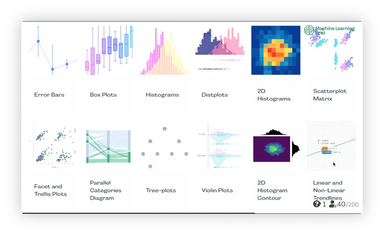
Plot categories
Histogram
px.histogram(data_frame=df, x="xColumn", title="My Title")
Stacked histogram (with more than one category)
px.histogram(df, x="xColumn", color="typeColumn", title="My Title")
Box Plot
px.box(df, y="columnName")
Stacked box plot (with more than one category)
px.box(df, y="dataColumn", x="categoryColumn")
Line Plot
px.line(df, x="date", y="price")
Stacked line plot
px.line(df, x="date", y="price", color="type")
Bar Plot
px.bar(df, x="price", y="region", orientation="h") # default: h(orizontal)
px.bar(df, x="region", y="price", orientation="v")
Stack bar plot
px.bar(df, x="price", y="region", color="type")
Stack side-by-side bar plot
px.bar(df, x="price", y="region", color="type", barmode="group")
Scatterplot
px.scatter(df, x="price", y="amount")
Enhancing plot styles
fig = px.bar(df_profit_per_city,
            y="city",
            x="profit",
            orientation="h",
            color="city",
            barmode='group',
            title="Plot Title",
            color_discrete_sequence=["red", "blue"]
      )

fig.update_layout(
    xaxis_title="profit (in €)",
    showlegend=False
    )

fig.show()
Geopandas
Resources
import numpy as np
import matplotlib.pyplot as plt #Plot
import pandas as pd	#DataFrames, Excel
import series as ser	#benummerte Columns
import geopandas as gpd
Python Mapping with GeoPandas
Data that comes with GeoPandas
world = gpd.read_file(gpd.datasets.get_path('naturalearth_lowres'))
Data structure
world.head()
Coordinate reference system (CRS)
world.crs
world.plot(color='grey', linewidth=0.5, edgecolor='white', figsize=(15,10))
Custom data (shape file)
import os
data_path = "../Data/"

cities = gpd.read_file(os.path.join(data_path, "ne_10m_populated_places.shp"))

cities.head()

cities.crs

cities.plot(figsize=(15,10), color='orange', markersize=5)
Join two geographical data sets
world.crs == cities.crs

base = world.plot(color='grey', linewidth=0.5, edgecolor='white', figsize=(15,10))
cities.plot(ax=base, color='orange', markersize=5)
base.set_axis_off()